Deep learning for the detection of γ-ray sources:
Bridging the gap between
training simulations and real telescope observations using unsupervised domain adaptation
DEPARTMENT OF ELECTRICAL AND COMPUTER ENGINEERING (NUS)
| Author | Under the supervision of |
| Michaël Dell'aiera (LAPP, LISTIC) | Thomas Vuillaume (LAPP) Alexandre Benoit (LISTIC) |



dellaiera.michael@gmail.com
Presentation outline
- Introduction
- The challenging transition from simulations to real data
- Data adaptation
- Multi-modality
- Domain adaptation
- Transformers
- Conclusion, perspectives
Introduction
Contextualisation
**[Cherenkov Telescope Array (CTA)](https://www.cta-observatory.org/)**
* Exploring the Universe at very high energies * γ-rays, powerful messenger to study the Universe * Next generation of ground-based observatories * Large-Sized Telescope-1 (LST-1) operational
**[GammaLearn](https://purl.org/gammalearn)**
* Collaboration between LAPP (CNRS) and LISTIC * Fosters innovative methods in AI for CTA * Evaluate the added value of deep learning * [Open-science](https://gitlab.in2p3.fr/gammalearn/gammalearn)
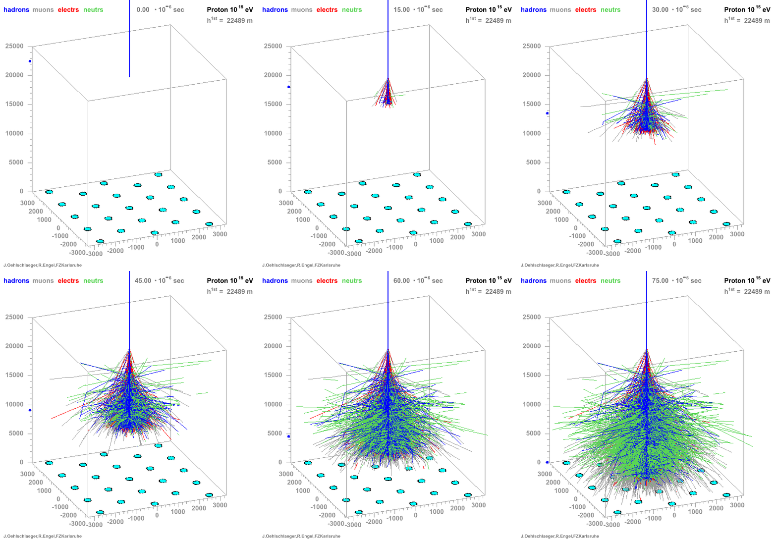
Fig. Principle of detection
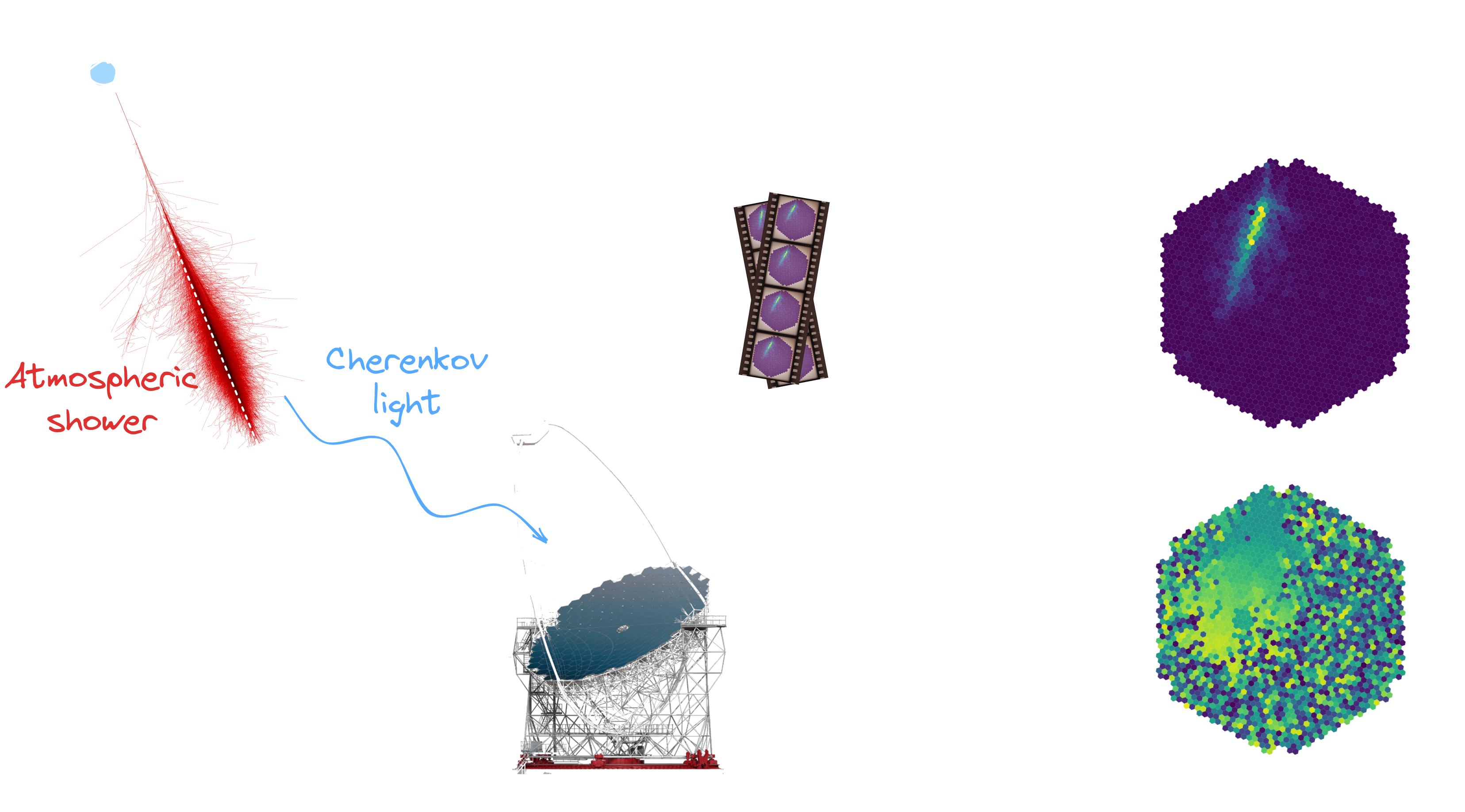
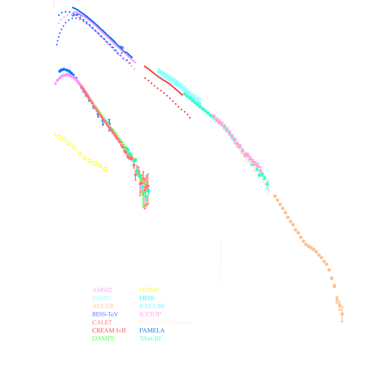
Particle distribution
**Many particles create atmospheric showers**

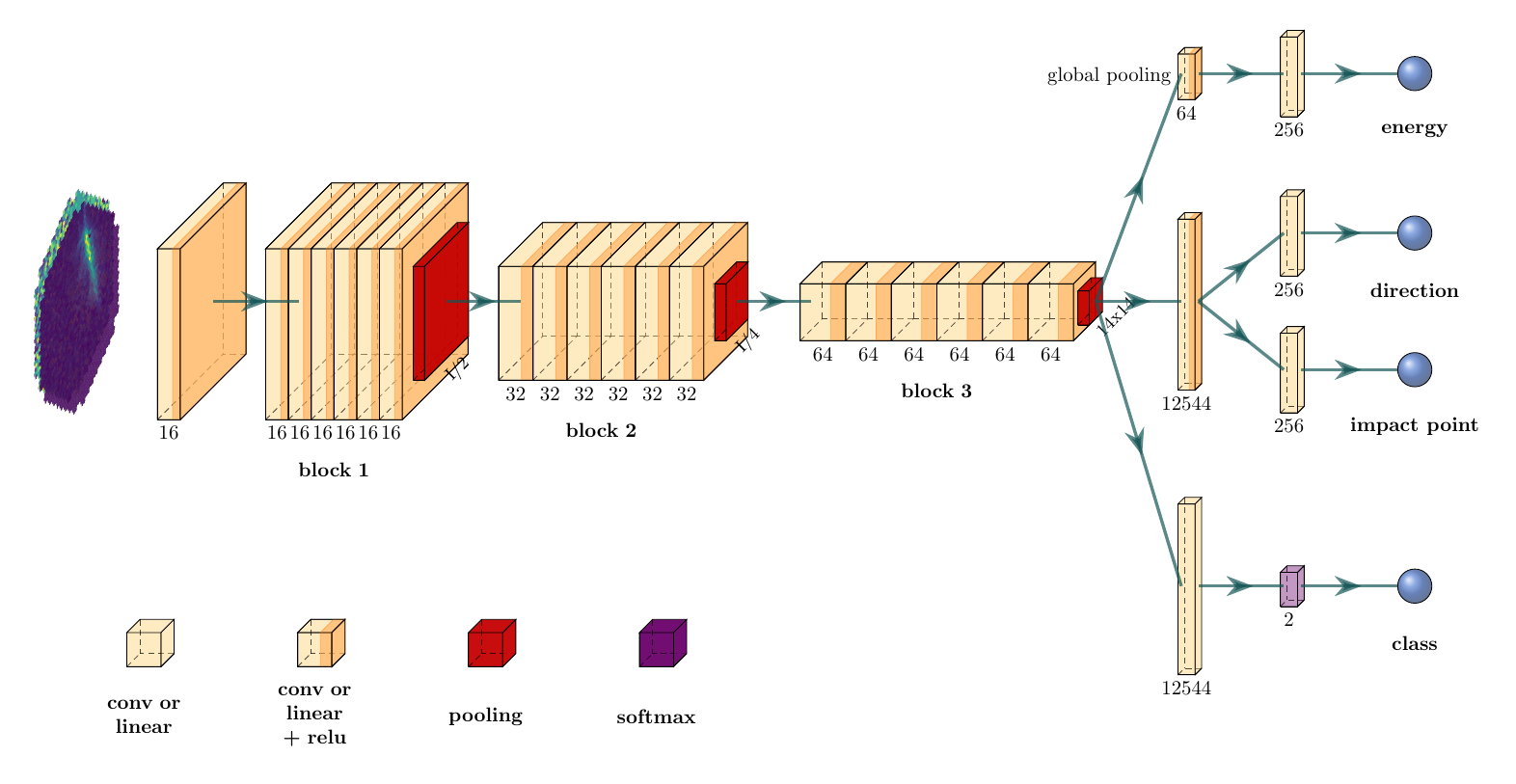
GammaLearn workflow
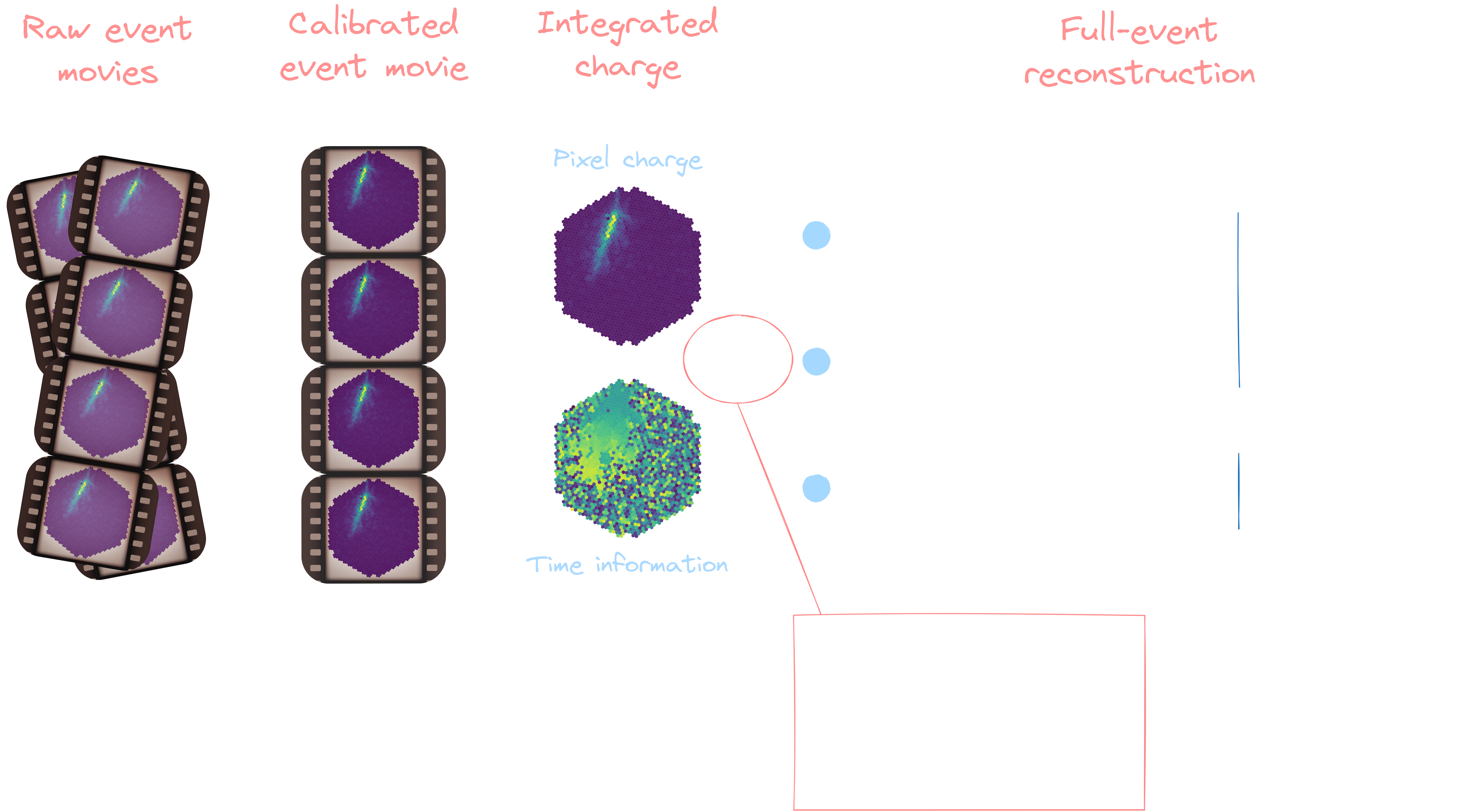
Physical attribute reconstruction
**Real labelled data are intrinsically unobtainable**
→ Training relying on simulations (Particle shower + instrument response)
* Machine learning * Morphological prior hypothesis: Ellipsoidal integrated signal * Image cleaning
GammaLearn* Deep learning (CNN-based) * No prior hypothesis * No image cleaning

The challenging transition from simulations to real data
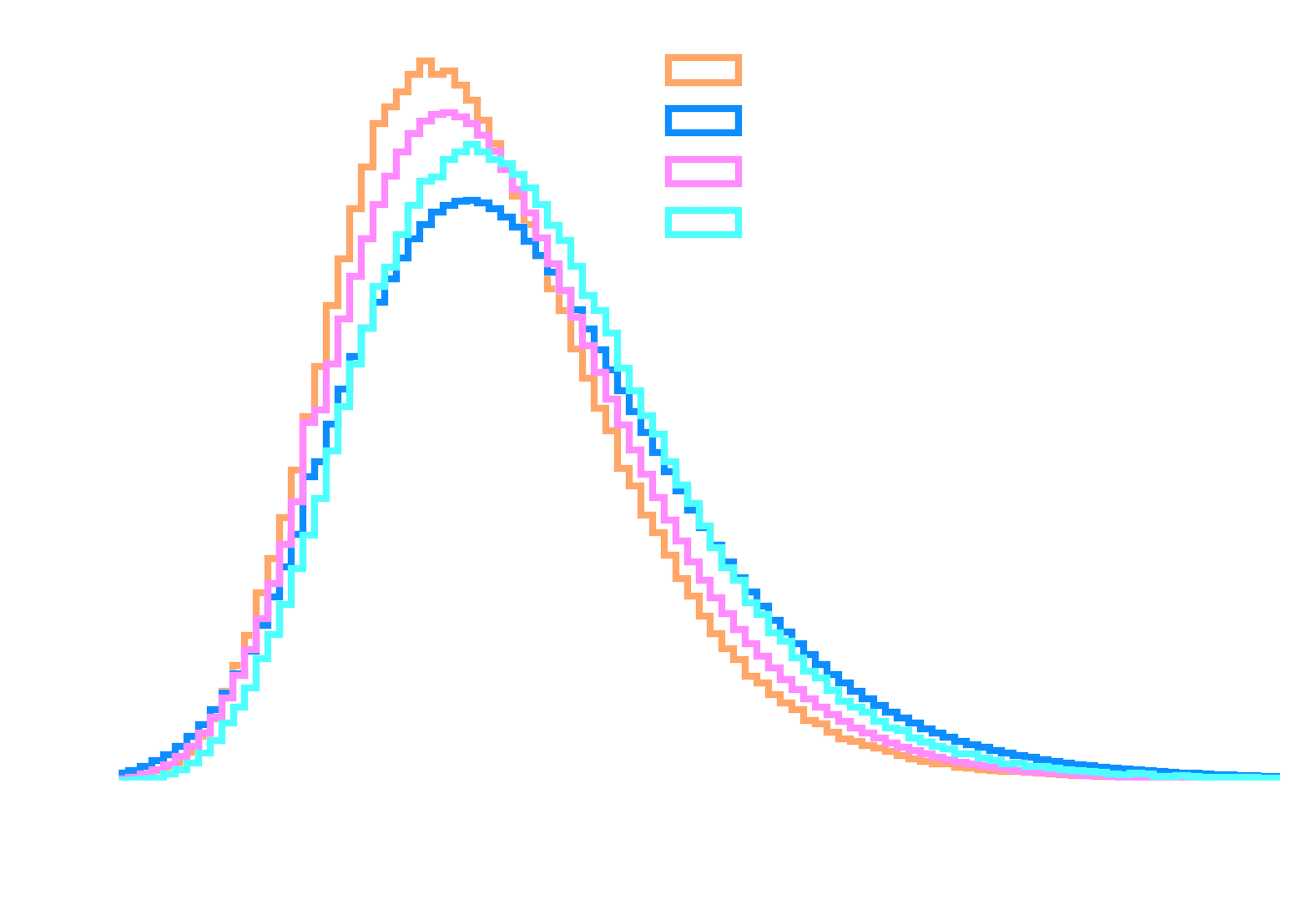
Simulations and real data discrepencies
**Simulations are approximations of the reality**


Simulations and real data discrepencies

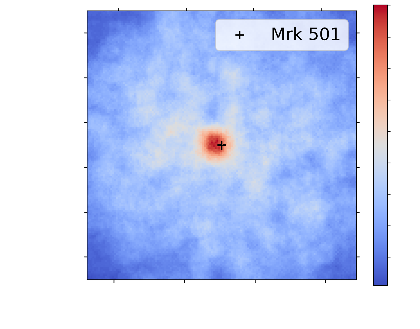
Data adaptation
Data adaptation
**Modify the simulations to fit the acquisitions**
Setup
Train |
Test |
| Labelled | Labelled |
MC+P(λ)
 ratio=50%/50% |
MC+P(λ)
 ratio=50%/50% |
Tab. Dataset composition
Results with data adaptation on simulations

Setup

Train |
Test |
| Labelled | Labelled |
MC+P(λ)
 ratio=50%/50% |
Real data ratio=1γ for > 1000p |
Tab. Dataset composition
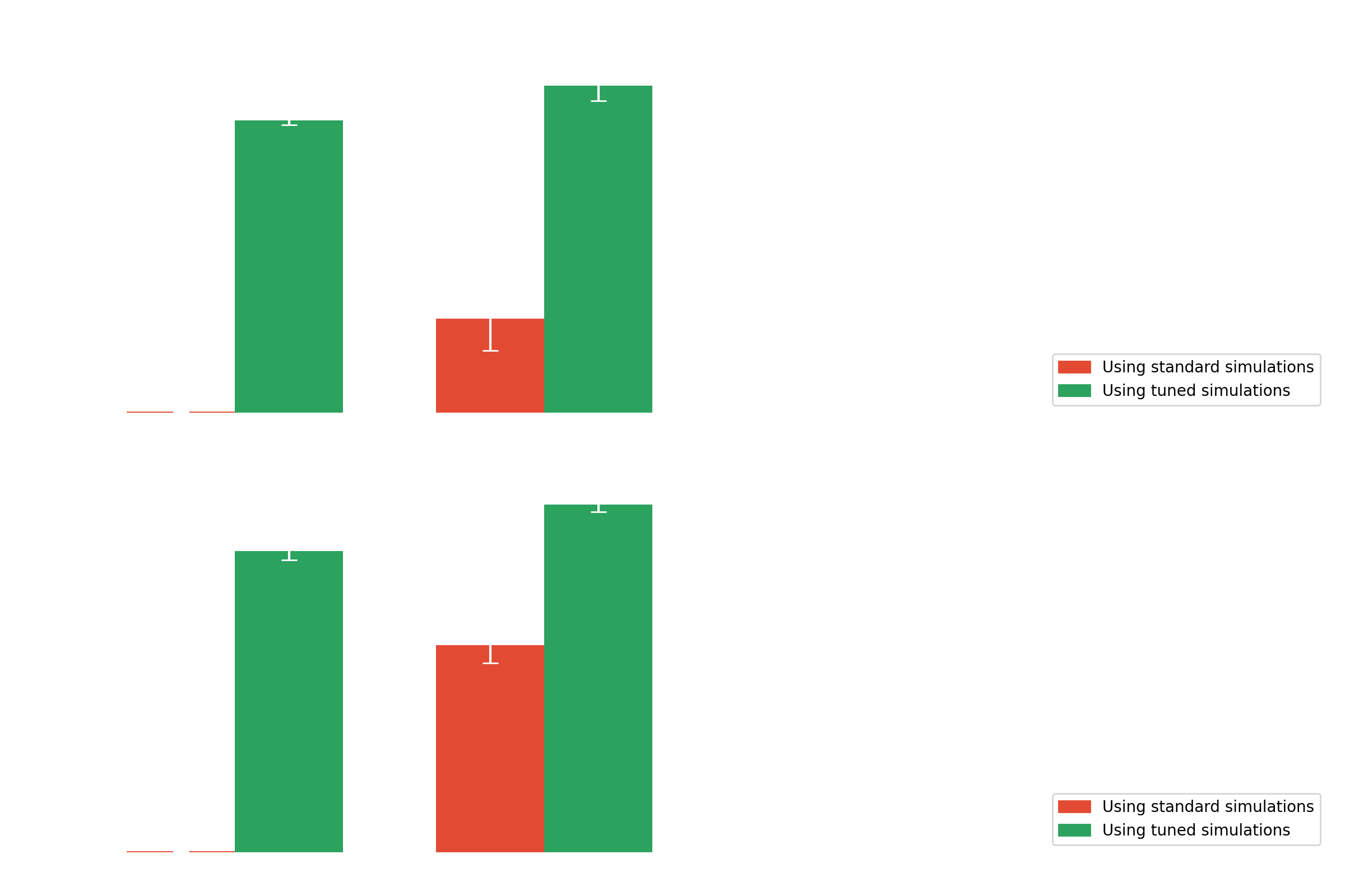
Results with data adaptation on Crab (real data)
Multi-modality
Multi-modality
**Modify the model to make it robust to noise**

Setup

Train |
Test |
| Labelled | Labelled |
MC+P(λ(t))
 ratio=50%/50% |
MC+P(λ)
 ratio=50%/50% |
Tab. Dataset composition
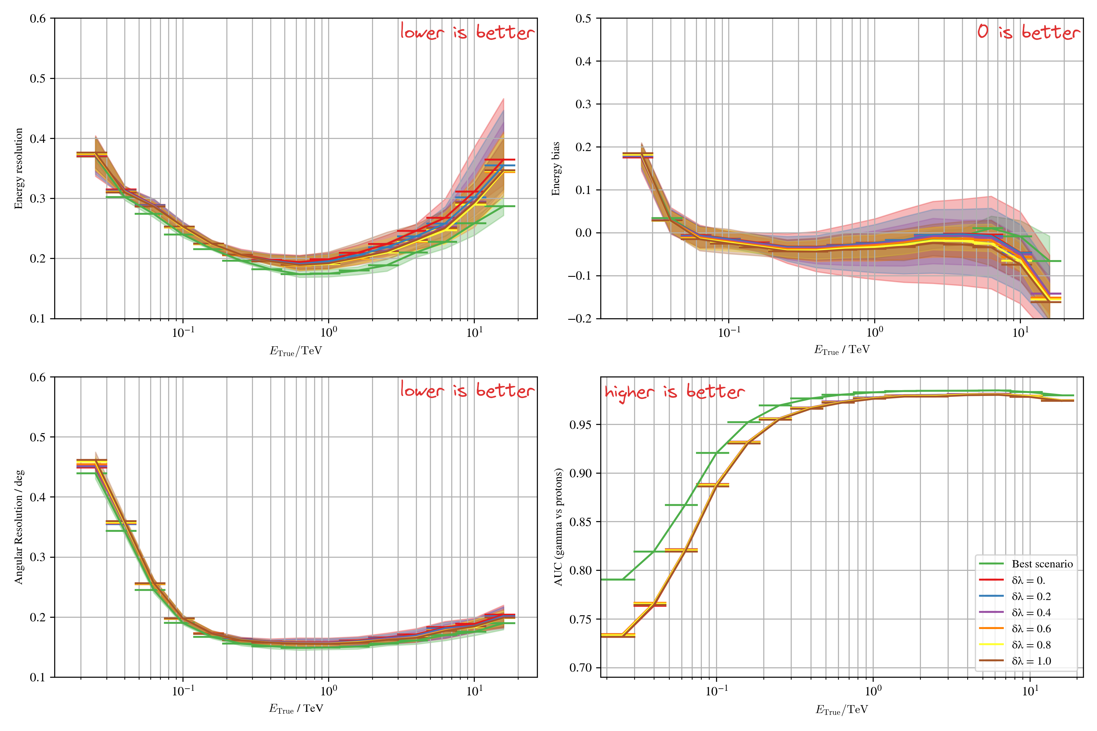
Results with multi-modality on simulations
Setup

Train |
Test |
| Labelled | Labelled |
MC+P(λ(t))
 ratio=50%/50% |
Real data ratio=1γ for > 1000p |
Tab. Dataset composition
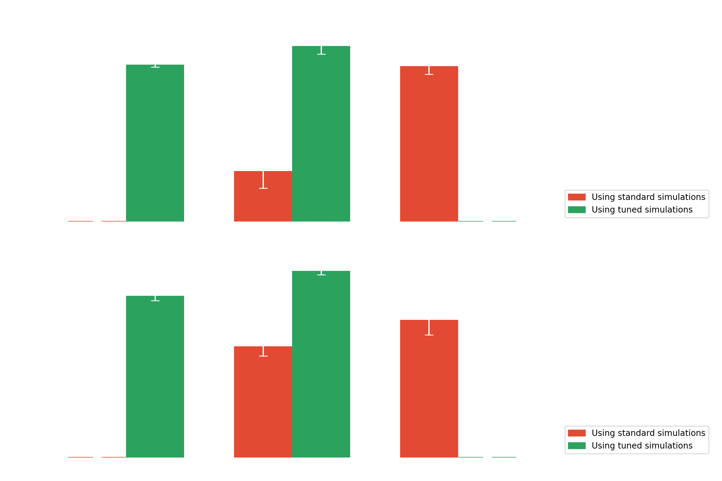
Results with multi-modality on Crab (real data)
Domain adaptation
Domain adaptation
**[Domain adaptation](https://arxiv.org/abs/2009.00155): Set of algorithms and techniques to reduce domain discrepancies**
* Take into account unknown differences between the source (labelled, simulations) and target (unlabelled, real data) domains * Somehow include unlabelled real data in the training * Selection, implementation and validation of [DANN](https://arxiv.org/abs/1505.07818) (focus of this talk), [DeepJDOT](https://arxiv.org/abs/1803.10081), [DeepCORAL](https://arxiv.org/abs/1607.01719)

Domain adaptation
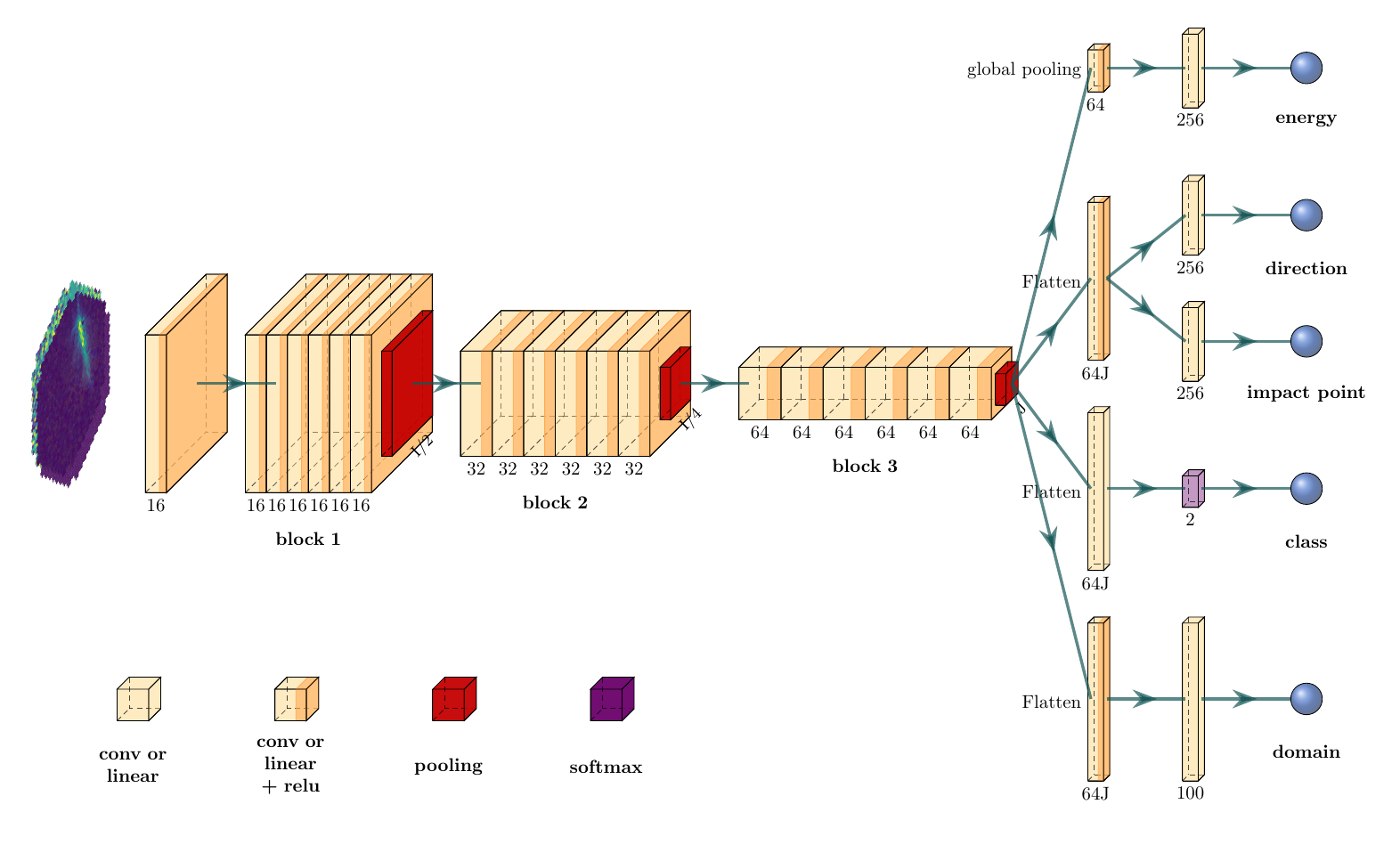
**Modify the model to make it domain agnostic**
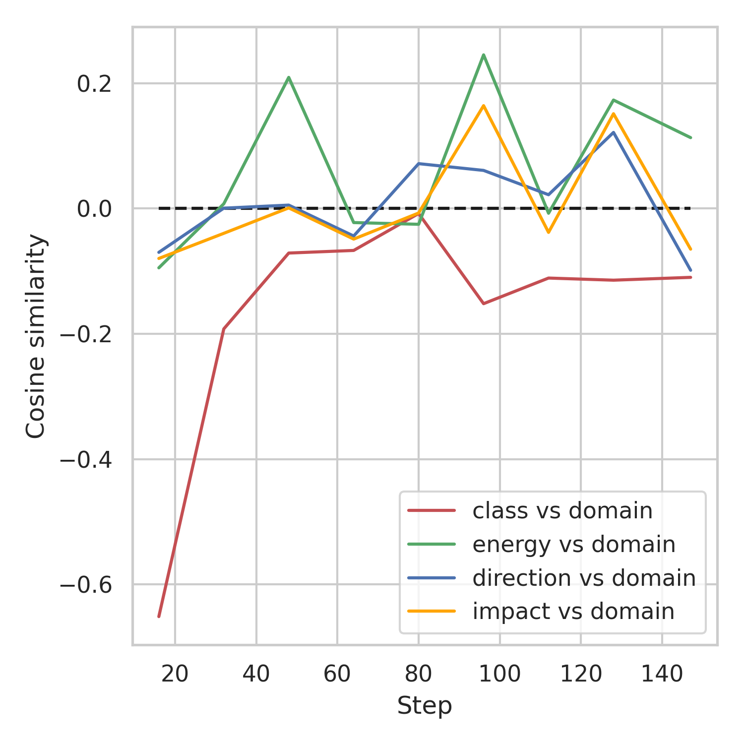
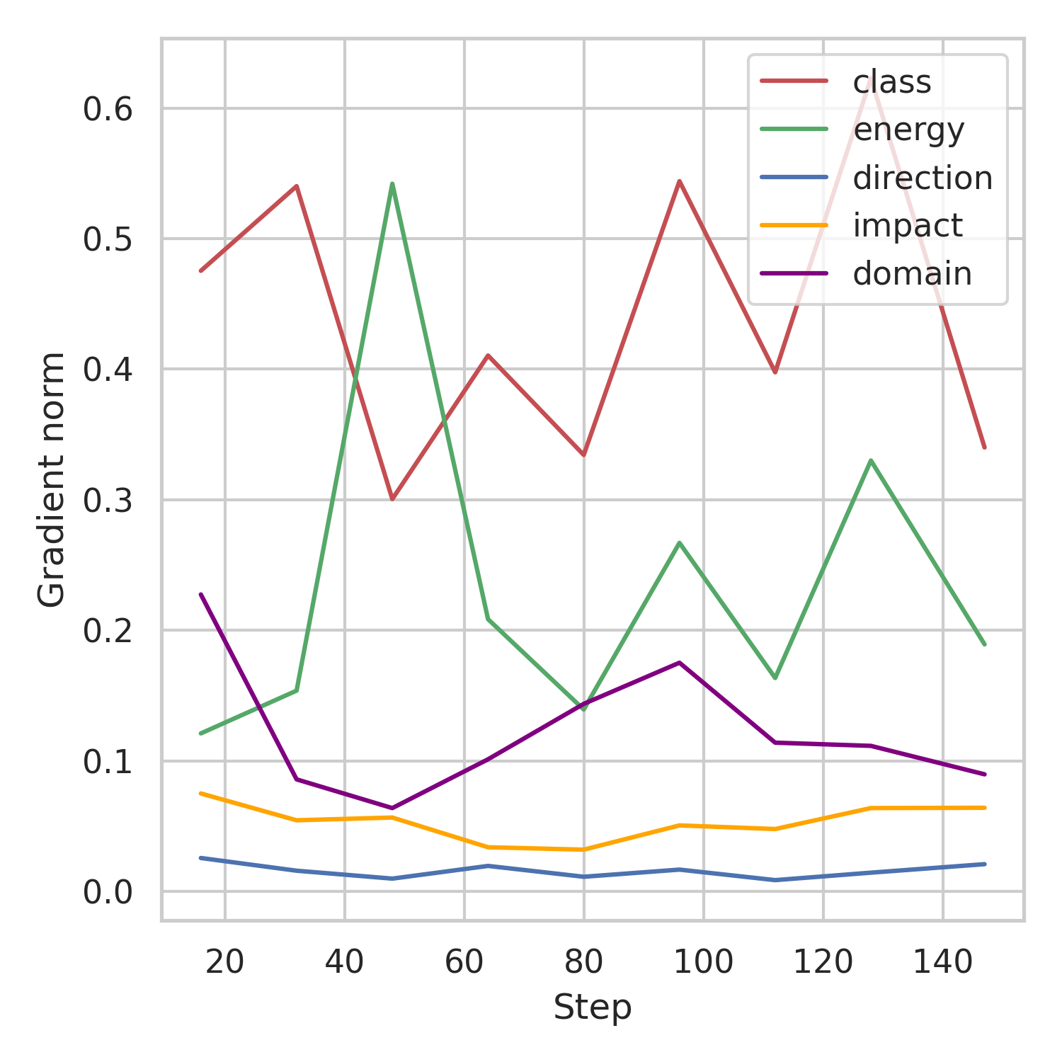
Multi-task balancing
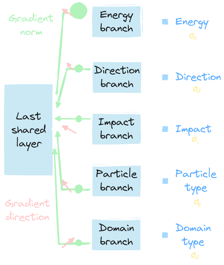
**[Multi-task balancing](https://arxiv.org/abs/1707.08114) (MTB): Simulateneous optimization of multiple tasks**
* In opposition to single-task learning * Correlated tasks help each other to learn better * Conflicting gradients (amplitude and/or direction) * Baseline: * Equal Weighting (EW) * Selection and implementation: * [Uncertainty Weighting](https://arxiv.org/abs/1705.07115) (UW) * [GradNorm](https://arxiv.org/abs/1711.02257) (GN)
Challenging multi-task optimization
Setup

Train |
Test |
|
| Source Labelled |
Target Unlabelled |
Unlabelled |
MC
 ratio=50%/50% |
MC+P(λ)
 ratio=50%/50% (No label shift) |
MC+P(λ)
 ratio=50%/50% |
Tab. Dataset composition
Results with domain adaptation on simulations
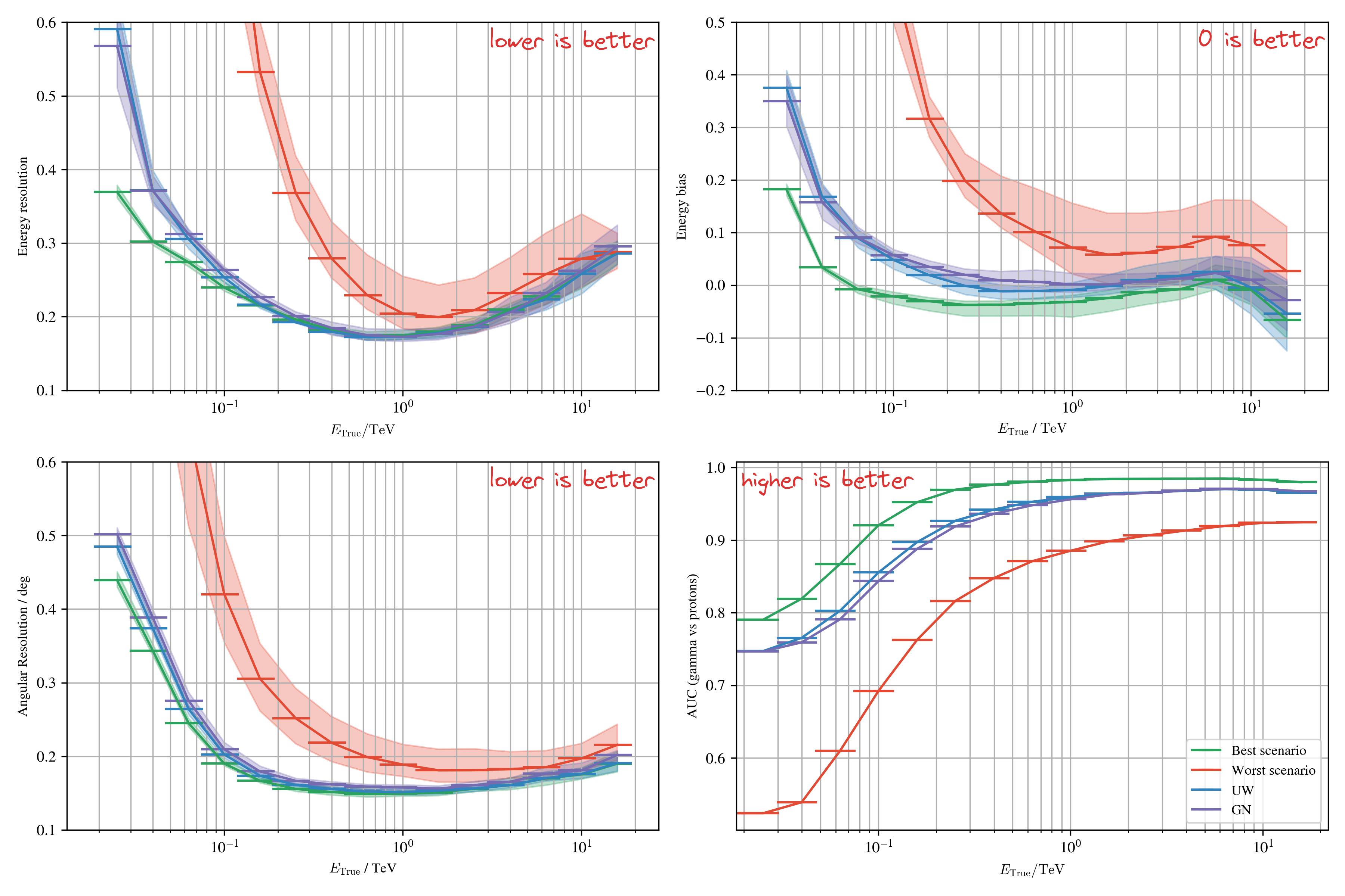
Setup

Train |
Test |
|
| Source Labelled |
Target Unlabelled |
Unlabelled |
MC
 ratio=50%/50% |
MC+P(λ)
 ratio=1γ for > 1000p (Label shift) |
MC+P(λ)
 ratio=50%/50% |
Tab. Dataset composition
Results with domain adaptation on simulations
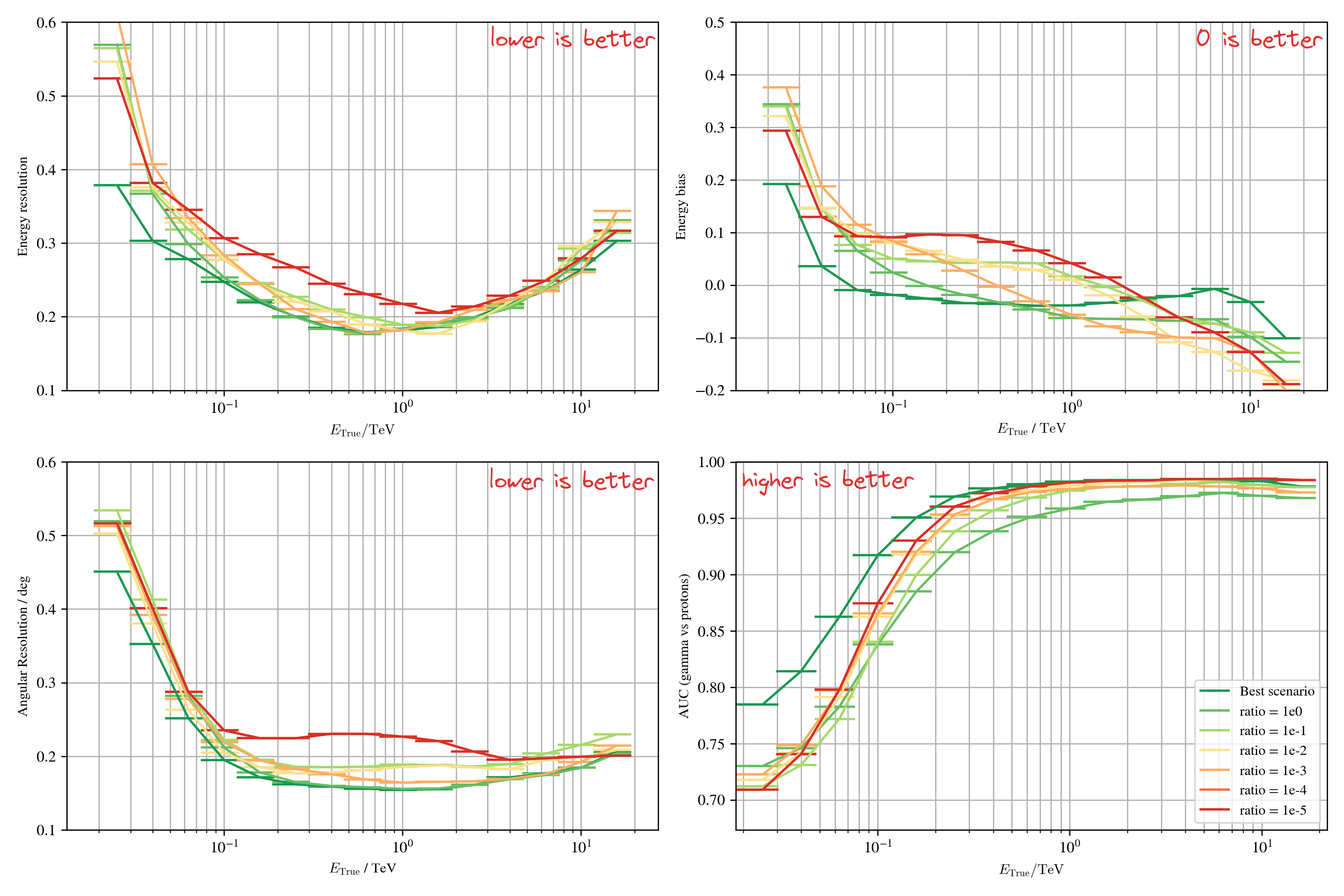
Conditional domain adaptation

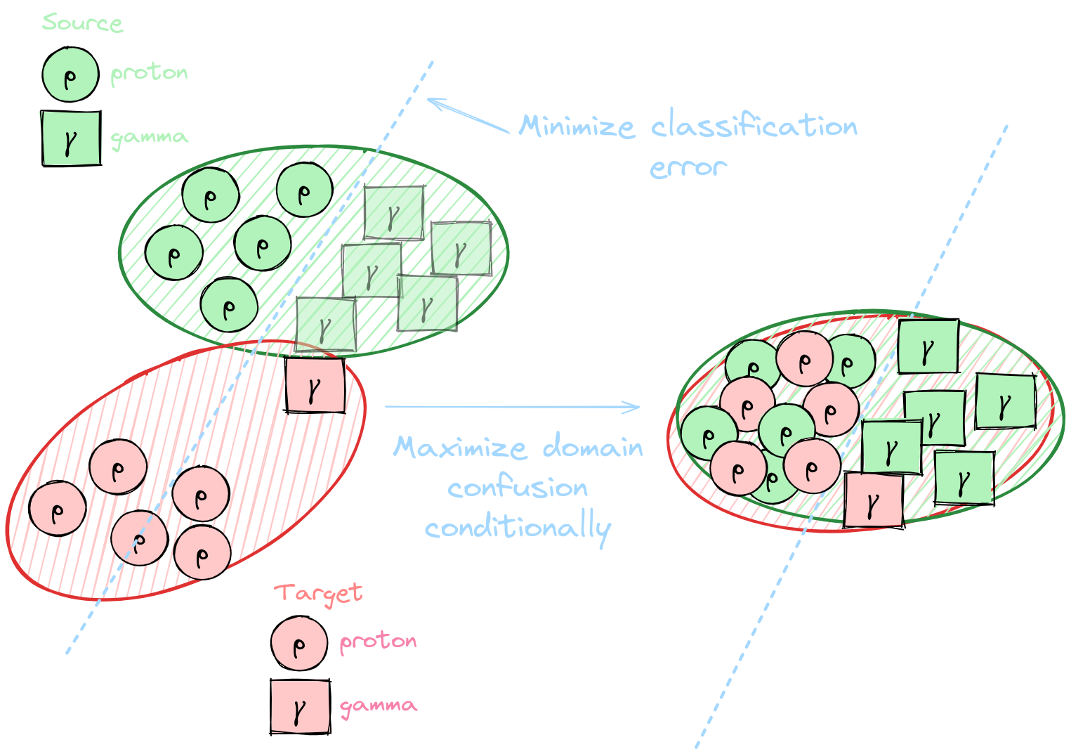
Results with domain adaptation on simulations
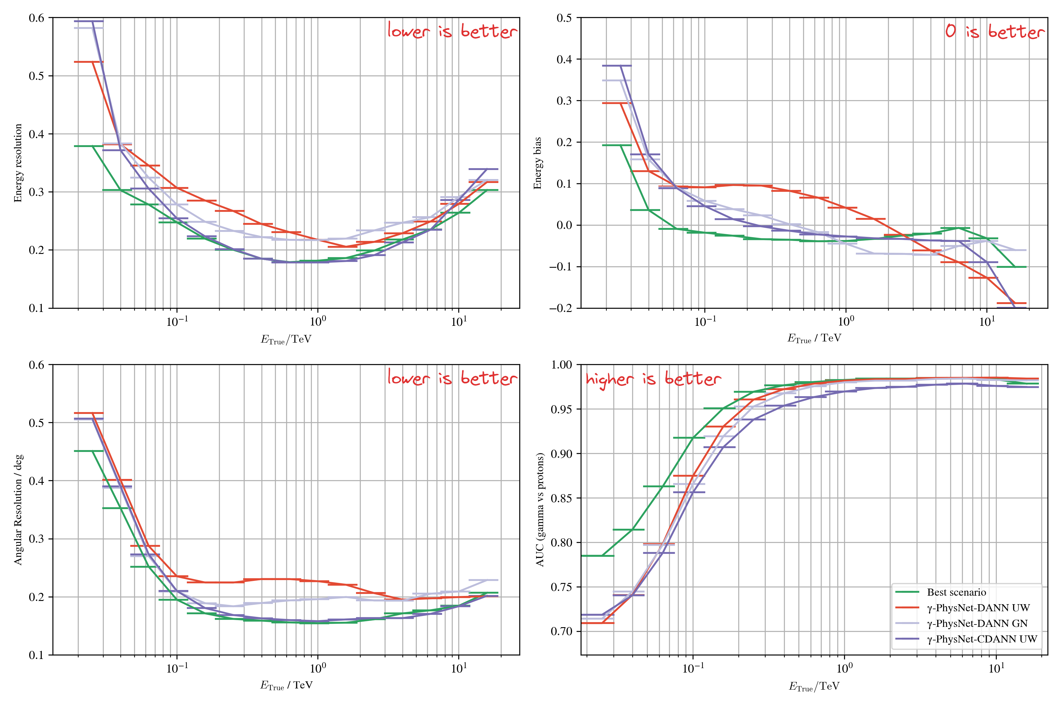
Setup
Train |
Test |
|
| Source Labelled |
Target Unlabelled |
Unlabelled |
MC+P(λ)
 ratio=50%/50% |
Real data ratio=1γ for > 1000p |
Real data ratio=1γ for > 1000p |
Tab. Dataset composition
Results with domain adaptation on Crab (real data)
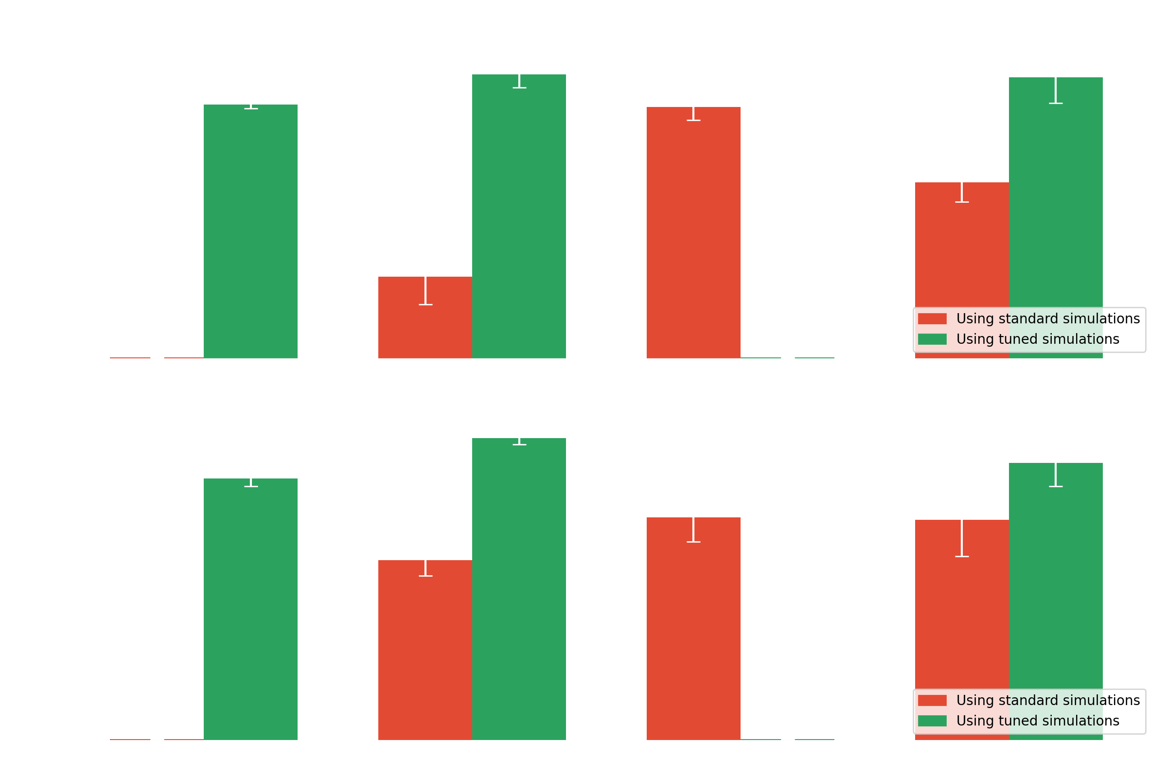
Transformers
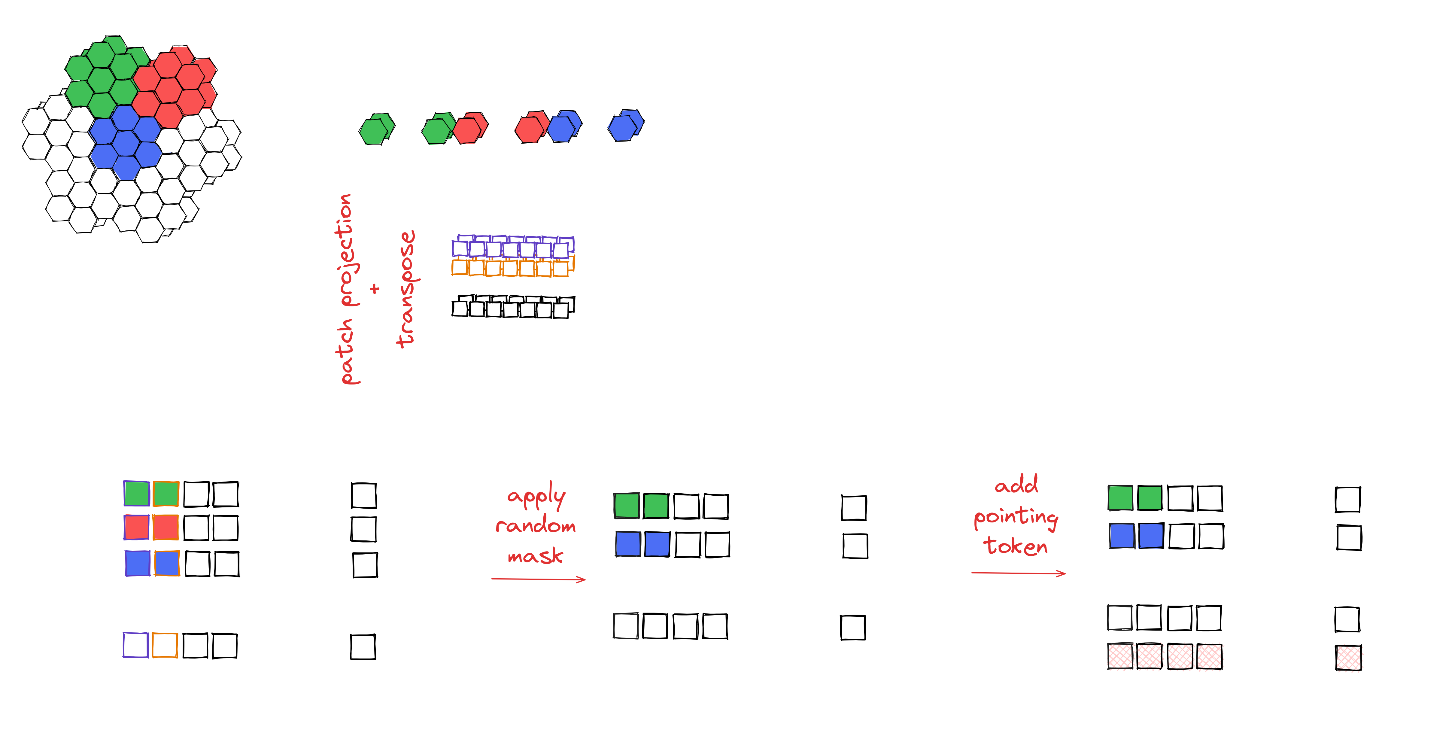
Masked Auto-Encoder (MAE)
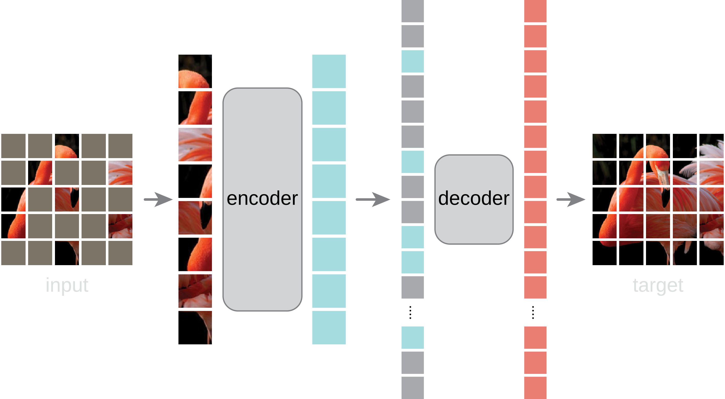
MAE applied to LST
Event reconstruction example 1

Event reconstruction example 2

Event reconstruction example 3

Event reconstruction example 4

Event reconstruction example 5

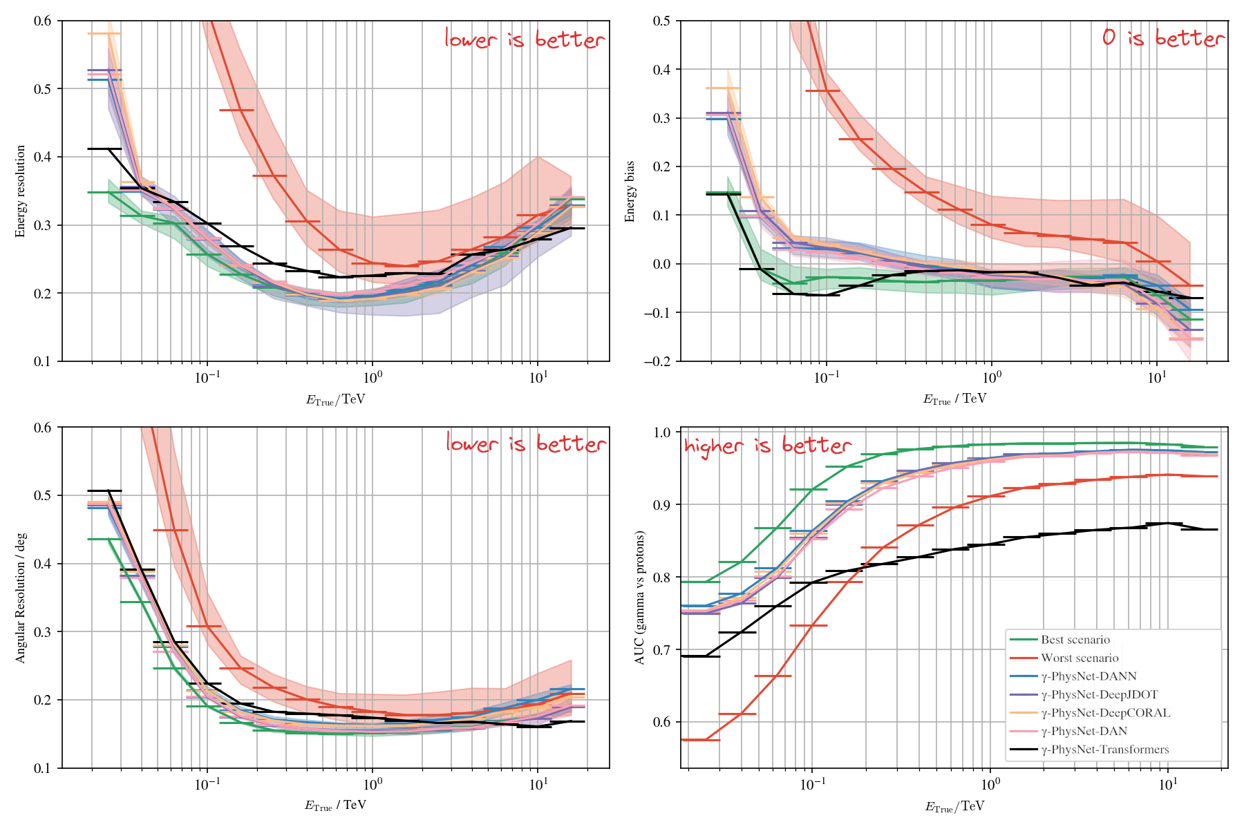
Results on simulations
Conclusion and perspectives
Conclusion & Perspectives
- Novel techniques (Multi-modality, Domain adaptation) to solve simulations vs real data discreprency
- Tested on simulations, in different settings (Light pollution and label shift)
- Tested on real data (Crab), both moonlight and no moonlight conditions
- Standard analysis and γ-PhysNet strongly affected by moonlight
- Data adaptation and multi-modality increase the performance in degraded conditions
- The benefits of domain adaptation are not well established yet
- Advantage demonstrated on MC data with different level of NSB
- Best results obtained on tuned data and on par with γ-PhysNet
- γ-PhysNet-CDANN allows to recover from label shift
- γ-PhysNet-CBN with pedestal image conditioning
- γ-PhysNet-Transformers with domain adaptation
- Generalization of the methods on other sources
Acknowledgments
![]()
![]()
![]()
![]()
![]()
![]()
![]()
![]()
![]()
![]()
![]()
![]()


